Elegant programming, part 1: introduction to Python
This I believe
I believe that the craft of scientific programming is as much about the correct and efficient implementation of numerical or algorithmic ideas as it is about their successful communication.
Communication to whom? Trivially, to the computer, who, as we know, is very literal minded and will do exactly what we tell it. But also to our collaborators, including our future selves, who will inspect and re-use the code; to other users in the scientific community, if (better, when!) the code is made publicly available; to referees at scientific journals, if (when!) an article is accompanied by the code used to produce its numbers and figures.
Mind you, I am not talking about code that cleverly embeds its own documentation (à la literate programming, or more modestly with something like doxygen's comment syntax), but about the code itself. I am partial to computer languages with expressive syntax that can be read immediately as the mathematics or algorithms that they embody. Indeed, I believe that beauty can serve as the first line of defense from confusion, complexity, and bugs. Beautiful code manifests the parallelism between a program and its mathematical and physical content; ugly code hides it and provide a breeding ground for inconsistencies and inefficiencies. Beautiful code can almost serve as its own documentation.
True, beauty is in the eye of the beholder [consider the wildly differing examples in the entertaining anthology Beautiful Code (Oram and Wilson 2007)], and every language seems beautiful and expressive to its expert practitioners.1 Yet, in the time (the 2010s) and context of this book (moderately collaborative scientific programming), I believe that there are combinations of computer language and coding style that appear beautiful, transparent, and expressive to most of us. One such combination is that of Python with the coding style best inspired by its Zen:
>>> import this
The Zen of Python, by Tim Peters

Beautiful is better than ugly.
Explicit is better than implicit.
Simple is better than complex.
Complex is better than complicated.
Flat is better than nested.
Sparse is better than dense.
Readability counts.
Special cases aren't special enough to break the rules.
Although practicality beats purity.
[...]
(Yes, you get the Zen by typing "import this" in the Python console.) How can you resist a language with its own Zen? More seriously, Python has much to recommend it to a computational scientist:
- It is expressive (Python/C = 6) and reflective.
- It is object-oriented, but casually so.
- It provides high-level mathematical–numerical objects and libraries.
- It can transparently wrap C and Fortran compiled code for high performance.
More important than any of this, programming in Python makes people happy. Python won't bother you with minutiae and lets you worry about the important things. It comes with batteries. Used mindfully, it lets you achieve a balance of expressive code and terse comments that tell the story of your computation.
So let's begin! I won't teach you Python (there are great books and tutorials for that), but I will show you what you can do with it, and you'll be able to learn it as we move along. And if you know Python already, enjoy the ride, and think about your progress toward its Nirvana.
(TO DO: SUGGEST PYTHON BOOKS AND TUTORIALS HERE.)
Goodbye C, hello Python
It's tradition to begin learning a computer language by writing a Hello World program. Although these days such an exercise seems silly, I suppose that it must originate from the time when it would take some careful punching of cards to get a room-sized computer to whirr satisfyingly, blinks its lights prettily, and finally produce the magic words on a console typewriter. Nevertheless, looking at the code that gets you the salute is not a bad way to get a first impression of the character of a computer language. Wikipedia helpfully lists Hello Worlds in many languages, go and have a look.
Python's character (friendly, terse, expressive) is exemplified well by comparing Hello World in Python and C. If you're an old C hand like me, these lines should flow automatically from your keyboard:
/* file helloworld.c */

#include <stdio.h>

int main(int argc,char **argv) {
    printf("Hello, World!\n");
}
We then compile and run the program:
$ gcc helloworld.c -o helloworld
$ ./helloworld
Hello, World!
(If you don't know C, don't worry: you'll be happy to see what you're not missing.) Hmm, it seems there's quite a bit of text there that is either unnecessary, or really meant for the computer rather than the programmer. Let's see:
- The statement
#include <stdio.h>tells the compiler that we're going to do some input/output, so the compiler should include all necessary function and constant definitions in the program. Fine... but printing to screen is so common that maybe this should be a default! - The function declaration
int main(int argc,char **argv)tells the compiler that this is indeed the code that should be run when entering the program; theargc/argvbusiness is about accessing command-line parameters, if any; and theintreturn type makes it possible to report back a success or failure to the shell wherehelloworldwas run. For such a simple program we don't need to do either! - The punctuation (
{,},;) shows the compiler where the code of themainfunction begins and end, and where each statement ends (there's only one here). Surely the compiler could be smarter and understand us without such punctiliousness! - Last,
printfstands for formatted print, and\nis a special character that starts a new line after what comes before. Isn't that what we would want most of the time, though?
(My apologies to Kernigan and Ritchie. They had very good reasons to make C as they did, and clearly it was a success. But the times have changed!)
We get Python by removing all this fluff from C: no #include <stdio.h>, no main declaration, no extra punctuation, no \n, but just
# file helloworld.py

print "Hello, World!"
We don't need to compile, but we call the Python interpreter directly:
$ python helloworld.py
Hello, World!
This must be close to the simplest that a Hello World program could be. And that's how it should be: precise enough that there's no room for misinterpretation, but without unnecessary cues for the computer that may only confuse humans (or the computer if they're left out).
In the cases where we do need to handle command-line parameters (for instance, get a personalized greeting), or pass a return code (0, for success) back to the shell, Python obliges happily. That functionality is part of the standard module sys:
# file helloyou.py

import sys

print "Hello,", sys.argv[1]
sys.exit(0)
which we run as
$ python helloyou.py Michele
Hello, Michele
Here importing sys gives us access ('.' = "member of") to the command-line parameters in the array sys.argv[] (just as in C, the first parameter sys.argv[0] is just the name of the program itself), and to the exit() function to pass back a return code.
The moral is that Python lets us include only the minimum amount of code necessary to obtain the functionality that we desire, and no more. In the rest of this section, we will see more interesting examples of Python's expressive syntax. No more saluting, though: we'll do some mathematics.
Pi, three ways
So we're going to use Python to compute the value of py (wait, pi). We'll proceed in the chronological order... and inverse order of numerical efficiency. Sometimes progress just isn't.
Pi by exhaustion
It seems fitting that we start with the first known algorithm to do so, devised by none other than Archimedes (circa 287–211 B.C.). He figured out that the perimeters of regular polygons inscribed and circumscribed around the unit circle would represent lower and higher bounds to \(2\pi\), of increasing accuracy as the number of sides increases. Using hexagons, the circumscribed semiperimeter comes to \(a_0 = 2 \sqrt{3}\), and the inscribed semiperimeter to \(b_0 = 3\).
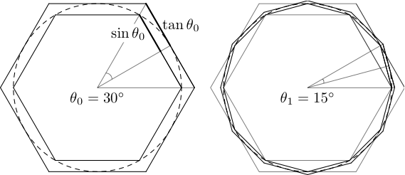
Archimedes' geometric scheme to approximate \(\pi\).
Using only geometric reasoning, Archimedes' was able to work out the change in the two perimeters when the number of sides is doubled, and he applied this step four times (up to 96-gons), obtaining \(b_4 < \pi < a_4\), namely \(\frac{223}{71} < \pi < \frac{22}{7}\), or \(3.1408 < \pi < 3.1429\). Archimedes didn't have decimal numbers, which makes his work even more remarkable.2 The iterative nature of the algorithm makes it possible to compute \(\pi\) (at least in principle) to any precision, and it can be rightfully said to mark the birth of both numerical and error analysis. Indeed, Archimedes' process of exhaustion anticipates modern integration... but that's another story.
From a modern viewpoint, it is hard to resist using trigonometry to reproduce Archimedes' doubling step, which in fact makes it quite painless. Given the perimeters
- \[a_n = 6 \times 2^n \, \tan \theta_n, \quad b_n = 6 \times 2^n \, \sin \theta_n, \quad \theta_n = \frac{\pi}{6 \times 2^n},\]
we need to find \(a_{n+1}\) and \(b_{n+1}\) given \(a_n\), \(b_n\). A quick look at our high-school trigonometry book suggests the bisection formulas,
- \[\tan \theta_{n+1} = \tan(\theta_n/2) = \frac{\sin \theta_n}{1 + \cos \theta_n}, \quad \sin \theta_{n+1} = \sin(\theta_n/2) = \pm \sqrt{\frac{1 - \cos \theta_n}{2}};\]
and after some rumination, we succeed in assembling
- \[a_{n+1} = \frac{2 a_n b_n}{a_n + b_n}, \quad b_{n+1} = \sqrt{a_{n+1} b_n}.\]
The iteration can be seeded with the hexagon (\(\theta_0 = \pi/6\), \(a_n = 2 \sqrt(3)\), \(b_n = 3\)). Let's try this out in Python:
# file archipi1.py

import math                       # get access to math functions

def archipi(n):
    a, b = 2 * math.sqrt(3), 3    # tuple unpacking

    for i in range(n):            # iterate from i = 0 to n-1, C-style
        a = 2 * a * b  / (a + b)
        b = math.sqrt(a * b)

    return a, b
We can run this function in the Python shell, and it works:
>>> import archipi1
>>> archipi1.archipi(10)
(3.1415929273850964, 3.1415925166921572)
So here we begin to see Python's expressive, no-nonsense syntax at work. The bodies of a function and of a loop, respectively, are identified by indentation (a tab or a consistent number of spaces), rather than braces. Variables don't need to be declared in advance, and their type is assigned dynamically at runtime. Variables can be assigned in pairs (or threes, or tuples) with a simple unpacking syntax.
Even more tellingly, the loop syntax for i in range(n): gets down to the point: we want to iterate over all values in a range. By contrast, C would have us worry about the details: we would write for (int i=0;i<n;i++) {...}, where we have to do all the dirty work of declaring a counter, incrementing it explicitly, and testing it against the upper limit. The Python syntax is even more general: as we shall see later in action, it supports for x in iterable, where x is any object that can yield a sequence of values. Indeed, range(n) is a built-in function that returns the list [0,1,...,n-1].
Let's see how fast archipi() converges:
>>> import math
>>> for i in range(24):
...     print archipi1.archipi(i)[0] - math.pi
...
0.322508961548
0.0737976555837
0.0180672885077
0.00449356154164
0.00112194605558
0.000280396390031
7.00934670554e-05
1.75230148964e-05
4.38073173292e-06
1.09518155833e-06
2.73795303318e-07
6.84488203895e-08
1.71122045423e-08
4.27805124659e-09
1.06951247858e-09
2.67377675556e-10
6.68434196882e-11
1.67101887882e-11
4.17665901864e-12
1.04360964315e-12
2.59792187762e-13
6.39488462184e-14
1.50990331349e-14
3.10862446895e-15
Here we've used the indexing notation to get the first element of the 2-tuples returned by archipi(). So we get roughly a digit every two iterations (i.e., the error decreases exponentially). We stop at the precision limit of Python's 64-bit floats. (The next iteration would report an error of zero, but that's a fluke, and it means only that we have matched the finite-precision value of the constant math.pi.)
Since we appreciate the beauty of mathematics, we should hold computer code to the same standards, so may refactor the very pragmatic archipi1 code into a more functional/mathematical style by separating the doubling step, the action of iterating the step,3 and the initial setup:
# file archipi2.py

import math

def archistep(a,b):
    a = 2 * a * b  / (a + b)
    b = math.sqrt(a * b)

    return a, b

# a general function to iterate func n times on x
def iterate(func,n,x):
    for i in range(n):
        x = func(*x)        # unpack the tuple x into two arguments

    return x

def archipi(n):
    return iterate(archistep,n,(2*math.sqrt(3),3))
Notably, we see that functions are first-class objects in Python, so it's OK to pass them as the argument of another function. The results of this code are the same as before, as it should be.
What if we want to push the computation beyond the 16 digits of double-precision floats? We need arbitrary-precision arithmetics, which is something that comes useful every now and then, so some helpful souls have created a Python package, mpmath, to do just that. (See the practical notes to learn how to install Python packages.)
We don't even need to change our code very much; it's sufficient to replace math with mpmath in archipi1/2, so that math.sqrt(3) begins its life as a special mpmath arbitrary-precision number. That mpmathness will spread, virus-like, to all the other numbers that are combined with it. We can do the replacement in the source code, or even interactively in the Python shell. Thus:
>>> import archipi, mpmath
>>> archipi.math = mpmath
>>> mpmath.mp.dps = 100             # set mpmath precision
>>> archipi2a.archipi(165)[0]
mpf('3.141592653589793238462643383279502884197169399375105820974944592307816406286208998628034825342117068094')
>>> archipi2.archipi(165)[0] - mpmath.pi
mpf('1.142987391282274982215783548305340959451909994822798661215125843227632635906738195675448021860172029649e-100')
Wow, uh? 165 iterations get us 100 digits. See Exercise 1 for an amazing variant of the Archimedes' algorithm that doubles the number of correct digits with every iteration.
Pi by persistence
We travel 1,900 years to Archimedes' future to find the Leibniz–Gregory series for the arctangent (Roy 1990),
- \[\arctan(x) = x - \frac{x^3}{3} + \frac{x^5}{5} - \frac{x^7}{7} + \cdots,\]
(which follows, e.g., by starting with \(\arctan(x) = \int dx/(1+x^2)\), using the geometric series \(1/(1 + x^2) = \sum_k x^{2k}\), and integrating) and therefore
- \[\arctan(1) = \frac{\pi}{4} = 1 - \frac{1}{3} + \frac{1}{5} - \frac{1}{7} \cdots.\]
Surely we can implement this easily in Python! A first, C-like attempt could be
# file seriespi1.py

def seriespi(n):
    sum = 0

    for k in range(0,n):
        sum = sum + (-1.0)**k/(2*k+1)    # ** is exponentiation in Python

    return 4 * sum
Here we have written \(-1\) as a floating-point number so that when it is divided by the integer 2*k+1, it returns a float, and not zero.4 However, this accumulator/loop update logic is not very natural in Python, where comprehensions are a much better way to generate lists. For example,
>>> [(-1.0)**k/(2*k+1) for k in range(5)]
[1.0, -0.33333333333333331, 0.20000000000000001, -0.14285714285714285, 0.1111111111111111]
and then we can use the built-in function sum:
>>> 4*sum([(-1.0)**k/(2*k+1) for k in range(200)])
3.1365926848388161
But if we're going to apply sum to the list, we may as well omit the brackets from the expression, which will give us a Python generator (an object that can be called repeatedly to yield a sequence of results). Thus we arrive at a very terse and math-like function:
# file seriespi2.py

def seriespi(n):
    return 4*sum((-1.0)**k/(2*k+1) for k in range(n))
Does it work?
>>> import seriespi2
>>> for i in range(0,2000,100):         # loop from 0 to 1999 in steps of 100
...     print i, seriespi2.seriespi(i)
...
0 0
100 3.13159290356
200 3.13659268484
300 3.13825932952
400 3.1390926575
500 3.13959265559
600 3.13992598808
700 3.14016408289
800 3.14034265408
900 3.14048154282
1000 3.14059265384
1100 3.14068356287
1200 3.1407593204
1300 3.14082342293
1400 3.14087836797
1500 3.140925987
1600 3.14096765365
1700 3.14100441835
1800 3.14103709808
1900 3.14106633784
Yes, but excruciatingly slowly! It takes the series 1000 terms to yield three decimal digits, and it seems to slow down after that. Indeed, the error decreases only as \(k^{-1}\), since the \(k\)-th residual is bounded by \(1/(2k+3)\). Those alternating signs are certainly to blame... see Exercise 2 for an acceleration transform that makes all signs positive, and improves the convergence of the series.
Pi by luck
In 1773, Georges-Louis Leclerc (the count of Buffon) posed what may have been the first problem in the field of geometric probability (Badger 1994). Supposing that we have a floor made of parallel strips of wood, and we drop a needle onto the floor, what is the probability that the needle will cross the boundary of a strip? Let's think about that.
For simplicity, let's say that the width of the strips and the length of the needle are both equal to one. We characterize a throw of the needle by the distance of the needle's tip from the strip boundary to the south (any \(x \in [0,1]\) is equally likely) and by the angle that the needle makes with respect to the strips (\(\theta = 0\) will be orthogonal, and by symmetry any \(\theta \in [0,2\pi]\) will be equally likely). For a given \(\theta\), the positions that yield a crossing will be those such that \(x + \sin \theta > 1\) (if \(\theta > 0\)) or \(x + \sin \theta < 0\) (if \(\theta < 0\)). It's easy to see that the fraction of such "good" positions is just \(|\sin \theta|\). Integrating this number over the distribution \(p(\theta) = 1/{2\pi}\) yields
- \[P(\mathrm{crossing}) = \frac{1}{2\pi} \int_0^{2\pi} |\sin \theta| d\theta = \frac{2}{\pi}.\]
Laplace later realized that Buffon's result could be used to provide an experimental determination of the value of \(\pi\). The number \(C\) of needle crossings in \(N\) throws would approximate \(\pi\) through \(C/N \simeq P(\mathrm{crossing}) = 2/\pi\), and therefore \(\pi \simeq 2 N/C\). This may have been another first... the birth of the Monte Carlo method, the very general idea of using random sampling to solve a deterministic problem.
A Python implementation is straightforward. All we need are random numbers between 0 and 1, which we can get from the random module:
# file buffonpi1.py

import random, math

# this function returns True if the needle falls across a boundary
def buffontrial():
    x, theta = random.random(), 2*math.pi*random.random()

    return not(0 < x + math.sin(theta) < 1)

def buffonpi(n):
    c = sum(buffontrial() for i in range(n))

    return 2.0 * n / c
Note Python's nice syntactic sugar for the double comparison in buffontrial(), and its flexibility in summing up boolean values (True and False in Python) as if they were ones and zeros.
This works, of course, but it converges even more slowly than the Leibniz series:
>>> import buffonpi1
>>> for i in range(10000,200000,10000):
...     print i, buffonpi1.buffonpi(i)
...
10000 3.10125600868
20000 3.16881882278
30000 3.14350081207
40000 3.15619205429
50000 3.15686460208
60000 3.14226609757
70000 3.14564328405
80000 3.13934780049
90000 3.15313737168
100000 3.13563175141
110000 3.13466224014
120000 3.1349190799
130000 3.13861828366
140000 3.13241150937
150000 3.14336906296
160000 3.14369639752
170000 3.14079055546
180000 3.15128808901
190000 3.14806683843
Indeed, on very general grounds one can show that the Monte Carlo error decreases as the standard deviation of the estimator (which in this case is \(2 N/C\)) divided by the square root of the number of samples. See Exercise 4 to derive this variance and use it to debunk a famous needle-throwing hoax.
Our Python code is already pretty clean, but given that we're at the end of the section, we can swagger a bit and do a one-liner version:
# file buffonpi2.py

import random, math

def buffonpi(n):
    return 2.0 * n / (n - sum(0 < random.random() + math.sin(2*math.pi*random.random()) < 1 for i in range(n)))
Exercises
Exercise 1 — Brent–Salamin
(TO COMPLETE.) The amazing Brent–Salamin algorithm is similar in spirit to Archimedes' exhaustion, but it doubles the number of correct digits of pi with every iteration. (MV: describe it.) Implement the algorithm using mpmath, and estimate the number of digits obtained after thirty iterations.
Exercise 2 — The digits of pi
(TO COMPLETE.) Now that you can generate pi digits ad libitum, look for patterns in their sequence and distribution. For instance, verify whether the distribution follows Zipf' law or is base-10 normal. Or find the second Feynman point (i.e., the sequence of six 9s that begins at decimal position 762; Feynman once said that he would like to memorize pi up to that point, so that could end his recitation with "nine, nine, nine, nine, nine, nine, and so on").
Exercise 3 – Lazzarini's lucky hand
In 1901, Mario Lazzarini claimed to have successfully determined \(\pi\) to six digits (3.1415929) using 3,408 Buffon throws (Badger 1994). This seems unlikely: the number \(C\) of throws that yield crossings is a Poisson variable with mean and variance equal to \(2 N/\pi\), and propagating the error to \(2N/C\) yields
\[\delta (2N/C) \simeq 2N/C^2 \delta C \simeq \frac{2N}{(2 N / \pi)^2} \sqrt{2 N/\pi} \simeq \sqrt{\frac{\pi^3}{2 N}}.\]
On this grounds alone, a few thousand throws should yield no more than one decimal digit. In addition, the number of throws (3,408) is very strange. Why not 3,500, or 4,000? The suspicion is that Lazzarini may have stopped throwing as soon as he chanced upon a lucky estimate, which is not fair, of course.
So we ask the question: if we keep updating our estimate of \(\pi\) as we accumulate throws, how close is it likely to wander to the correct value? For exercise, adapt the buffonpi1 code to determine the closest approach over a sequence of throws, and then run it repeatedly to understand the statistics of Lazzarini's cheat. In the light of those, do you think that his cheating was of an even worse kind?
References, references
Badger, L. 1994. “Lazzarini’s Lucky Approximation of pi.” Mathematics Magazine 67: 83-91.
Ifrah, G. 2000. The Universal History of Numbers. Hoboken, NJ: John Wiley and Sons.
Oram, Andy, and Greg Wilson. 2007. Beautiful Code: Leading Programmers Explain How They Think. Sebastopol, CA: O’Reilly.
Roy, R. 1990. “The discovery of the series formula for pi by Leibniz, Gregory and Nilakantha.” Mathematics Magazine 63: 291-306.
Even Lisp: when I asked Gerald Jay Sussman, of [Structure and Interpretation] fame, whether he didn't mind all the parentheses overrunning his code (certainly a FAQ), he replied that he didn't even really see those anymore. ↩
The difficulty in doing arithmetics prior to the positional notation is witnessed by the advice given to a wealthy 16th-century German merchant about the choice of a college for his son: "If you only want him to be able to cope with addition and subtraction, then any French or German university will do. But [for] multiplication and division—assuming that he has sufficient gifts—then you will have to send him to Italy." (Ifrah 2000) ↩
There's a wart in this
iterate()function, which uses the Python*notation to unpack a tuple into the separate arguments needed byarchistep(). This would not work iffunc()takes a single argument; the simplest way of fixing it would be to check ifxis a sequence (TO DO: how?) and then callfunc(*x)orfunc(x)depending on the result. ↩This is an infamous C pitfall that is remedied in Python 3, where, for instance,
1/2is0.5. The same behavior can be obtained in Python 2.x with the statementfrom __future__ import division. As in many things Pythonic, enabling backported features comes with a touch of humor. ↩